What Is A Matched Filter

Filters used in signal processing that are optimal in some sense.

In signal processing, a matched filter is obtained by correlating a known delayed indicate, or template, with an unknown point to notice the presence of the template in the unknown signal.^{[1] [ii]} This is equivalent to convolving the unknown signal with a conjugated time-reversed version of the template. The matched filter is the optimal linear filter for maximizing the betoken-to-noise ratio (SNR) in the presence of condiment stochastic racket.

Matched filters are normally used in radar, in which a known betoken is sent out, and the reflected signal is examined for common elements of the out-going signal. Pulse compression is an example of matched filtering. Information technology is and so called considering the impulse response is matched to input pulse signals. Two-dimensional matched filters are commonly used in image processing, e.g., to ameliorate the SNR of X-ray observations. Matched filtering is a demodulation technique with LTI (linear time invariant) filters to maximize SNR.^[3] It was originally also known as a Due north filter.^[4]

Derivation [edit]

Derivation via matrix algebra [edit]

The post-obit section derives the matched filter for a discrete-fourth dimension system. The derivation for a continuous-fourth dimension system is like, with summations replaced with integrals.

The matched filter is the linear filter, ${\displaystyle h}$ , that maximizes the output signal-to-noise ratio.

${\displaystyle \ y[n]=\sum _{m=-\infty }^{\infty }h[northward-k]10[g],}$

where ${\displaystyle x[thousand]}$ is the input equally a function of the independent variable ${\displaystyle k}$ , and ${\displaystyle y[n]}$ is the filtered output. Though nosotros nearly often express filters every bit the impulse response of convolution systems, as above (see LTI arrangement theory), it is easiest to think of the matched filter in the context of the inner product, which we will see shortly.

We can derive the linear filter that maximizes output signal-to-racket ratio past invoking a geometric statement. The intuition behind the matched filter relies on correlating the received betoken (a vector) with a filter (another vector) that is parallel with the signal, maximizing the inner production. This enhances the signal. When we consider the additive stochastic noise, we have the additional claiming of minimizing the output due to racket past choosing a filter that is orthogonal to the racket.

Let united states of america formally ascertain the trouble. Nosotros seek a filter, ${\displaystyle h}$ , such that we maximize the output signal-to-noise ratio, where the output is the inner product of the filter and the observed signal ${\displaystyle 10}$ .

Our observed bespeak consists of the desirable signal ${\displaystyle s}$ and additive noise ${\displaystyle v}$ :

${\displaystyle \ x=south+v.\,}$

Let the states define the covariance matrix of the dissonance, reminding ourselves that this matrix has Hermitian symmetry, a holding that will become useful in the derivation:

${\displaystyle \ R_{v}=Eastward\{vv^{\mathrm {H} }\}\,}$

where ${\displaystyle 5^{\mathrm {H} }}$ denotes the cohabit transpose of ${\displaystyle five}$ , and ${\displaystyle E}$ denotes expectation. Let us phone call our output, ${\displaystyle y}$ , the inner production of our filter and the observed signal such that

${\displaystyle \ y=\sum _{1000=-\infty }^{\infty }h^{*}[m]10[thousand]=h^{\mathrm {H} }x=h^{\mathrm {H} }s+h^{\mathrm {H} }five=y_{s}+y_{v}.}$

Nosotros at present define the signal-to-noise ratio, which is our objective part, to be the ratio of the power of the output due to the desired signal to the power of the output due to the noise:

${\displaystyle \mathrm {SNR} ={\frac {|y_{due south}|^{2}}{Due east\{|y_{v}|^{2}\}}}.}$

We rewrite the to a higher place:

${\displaystyle \mathrm {SNR} ={\frac {|h^{\mathrm {H} }due south|^{2}}{East\{|h^{\mathrm {H} }v|^{2}\}}}.}$

Nosotros wish to maximize this quantity past choosing ${\displaystyle h}$ . Expanding the denominator of our objective function, we accept

${\displaystyle \ E\{|h^{\mathrm {H} }v|^{ii}\}=E\{(h^{\mathrm {H} }v){(h^{\mathrm {H} }v)}^{\mathrm {H} }\}=h^{\mathrm {H} }East\{vv^{\mathrm {H} }\}h=h^{\mathrm {H} }R_{5}h.\,}$

Now, our ${\displaystyle \mathrm {SNR} }$ becomes

${\displaystyle \mathrm {SNR} ={\frac {|h^{\mathrm {H} }s|^{2}}{h^{\mathrm {H} }R_{v}h}}.}$

Nosotros volition rewrite this expression with some matrix manipulation. The reason for this seemingly counterproductive measure will go evident shortly. Exploiting the Hermitian symmetry of the covariance matrix ${\displaystyle R_{v}}$ , nosotros can write

${\displaystyle \mathrm {SNR} ={\frac {|{(R_{v}^{1/2}h)}^{\mathrm {H} }(R_{v}^{-i/two}south)|^{ii}}{{(R_{v}^{1/2}h)}^{\mathrm {H} }(R_{five}^{1/2}h)}},}$

Nosotros would like to find an upper bound on this expression. To exercise so, nosotros first recognize a form of the Cauchy–Schwarz inequality:

${\displaystyle \ |a^{\mathrm {H} }b|^{2}\leq (a^{\mathrm {H} }a)(b^{\mathrm {H} }b),\,}$

which is to say that the square of the inner product of 2 vectors tin merely be as big equally the production of the private inner products of the vectors. This concept returns to the intuition behind the matched filter: this upper bound is achieved when the two vectors ${\displaystyle a}$ and ${\displaystyle b}$ are parallel. We resume our derivation by expressing the upper bound on our ${\displaystyle \mathrm {SNR} }$ in low-cal of the geometric inequality to a higher place:

${\displaystyle \mathrm {SNR} ={\frac {|{(R_{v}^{1/2}h)}^{\mathrm {H} }(R_{v}^{-one/2}south)|^{ii}}{{(R_{v}^{i/two}h)}^{\mathrm {H} }(R_{v}^{1/two}h)}}\leq {\frac {\left[{(R_{v}^{1/2}h)}^{\mathrm {H} }(R_{v}^{1/2}h)\correct]\left[{(R_{five}^{-ane/ii}due south)}^{\mathrm {H} }(R_{v}^{-1/2}s)\right]}{{(R_{five}^{1/ii}h)}^{\mathrm {H} }(R_{5}^{ane/2}h)}}.}$

Our valiant matrix manipulation has now paid off. Nosotros see that the expression for our upper leap tin can be greatly simplified:

${\displaystyle \mathrm {SNR} ={\frac {|{(R_{v}^{1/two}h)}^{\mathrm {H} }(R_{v}^{-1/two}s)|^{2}}{{(R_{v}^{ane/ii}h)}^{\mathrm {H} }(R_{v}^{ane/2}h)}}\leq s^{\mathrm {H} }R_{five}^{-1}s.}$

Nosotros can achieve this upper spring if we choose,

${\displaystyle \ R_{v}^{one/2}h=\alpha R_{v}^{-1/2}s}$

where ${\displaystyle \alpha }$ is an arbitrary existent number. To verify this, we plug into our expression for the output ${\displaystyle \mathrm {SNR} }$ :

${\displaystyle \mathrm {SNR} ={\frac {|{(R_{v}^{1/2}h)}^{\mathrm {H} }(R_{five}^{-1/two}s)|^{ii}}{{(R_{v}^{1/two}h)}^{\mathrm {H} }(R_{v}^{1/2}h)}}={\frac {\alpha ^{ii}|{(R_{v}^{-1/two}s)}^{\mathrm {H} }(R_{v}^{-1/2}southward)|^{2}}{\alpha ^{ii}{(R_{five}^{-1/ii}s)}^{\mathrm {H} }(R_{v}^{-i/two}s)}}={\frac {|s^{\mathrm {H} }R_{v}^{-one}s|^{2}}{s^{\mathrm {H} }R_{v}^{-one}southward}}=s^{\mathrm {H} }R_{v}^{-1}s.}$

Thus, our optimal matched filter is

${\displaystyle \ h=\alpha R_{v}^{-1}s.}$

We often cull to normalize the expected value of the power of the filter output due to the noise to unity. That is, nosotros constrain

${\displaystyle \ E\{|y_{v}|^{2}\}=1.\,}$

This constraint implies a value of ${\displaystyle \blastoff }$ , for which we can solve:

${\displaystyle \ Due east\{|y_{five}|^{ii}\}=\alpha ^{2}southward^{\mathrm {H} }R_{v}^{-1}s=i,}$

yielding

${\displaystyle \ \alpha ={\frac {1}{\sqrt {due south^{\mathrm {H} }R_{v}^{-i}southward}}},}$

giving united states of america our normalized filter,

${\displaystyle \ h={\frac {ane}{\sqrt {s^{\mathrm {H} }R_{5}^{-1}s}}}R_{v}^{-1}s.}$

If nosotros care to write the impulse response ${\displaystyle h}$ of the filter for the convolution system, it is simply the complex cohabit time reversal of the input ${\displaystyle s}$ .

Though nosotros accept derived the matched filter in discrete time, nosotros tin extend the concept to continuous-time systems if nosotros replace ${\displaystyle R_{v}}$ with the continuous-fourth dimension autocorrelation office of the racket, assuming a continuous signal ${\displaystyle s(t)}$ , continuous noise ${\displaystyle v(t)}$ , and a continuous filter ${\displaystyle h(t)}$ .

Derivation via Lagrangian [edit]

Alternatively, we may solve for the matched filter by solving our maximization trouble with a Lagrangian. Again, the matched filter endeavors to maximize the output point-to-noise ratio ( ${\displaystyle \mathrm {SNR} }$ ) of a filtered deterministic point in stochastic additive racket. The observed sequence, again, is

${\displaystyle \ x=s+five,\,}$

with the noise covariance matrix,

${\displaystyle \ R_{v}=East\{vv^{\mathrm {H} }\}.\,}$

The signal-to-noise ratio is

${\displaystyle \mathrm {SNR} ={\frac {|y_{southward}|^{2}}{E\{|y_{v}|^{2}\}}},}$

where ${\displaystyle y_{due south}=h^{\mathrm {H} }south}$ and ${\displaystyle y_{v}=h^{\mathrm {H} }v}$ .

Evaluating the expression in the numerator, we take

${\displaystyle \ |y_{s}|^{2}={y_{south}}^{\mathrm {H} }y_{s}=h^{\mathrm {H} }ss^{\mathrm {H} }h.\,}$

and in the denominator,

${\displaystyle \ E\{|y_{v}|^{ii}\}=E\{{y_{five}}^{\mathrm {H} }y_{five}\}=E\{h^{\mathrm {H} }vv^{\mathrm {H} }h\}=h^{\mathrm {H} }R_{five}h.\,}$

The signal-to-noise ratio becomes

${\displaystyle \mathrm {SNR} ={\frac {h^{\mathrm {H} }ss^{\mathrm {H} }h}{h^{\mathrm {H} }R_{v}h}}.}$

If we now constrain the denominator to exist 1, the problem of maximizing ${\displaystyle \mathrm {SNR} }$ is reduced to maximizing the numerator. We tin then codify the problem using a Lagrange multiplier:

${\displaystyle \ h^{\mathrm {H} }R_{v}h=ane}$

${\displaystyle \ {\mathcal {L}}=h^{\mathrm {H} }ss^{\mathrm {H} }h+\lambda (i-h^{\mathrm {H} }R_{v}h)}$

${\displaystyle \ \nabla _{h^{*}}{\mathcal {L}}=ss^{\mathrm {H} }h-\lambda R_{v}h=0}$

${\displaystyle \ (ss^{\mathrm {H} })h=\lambda R_{v}h}$

which we recognize every bit a generalized eigenvalue problem

${\displaystyle \ h^{\mathrm {H} }(ss^{\mathrm {H} })h=\lambda h^{\mathrm {H} }R_{v}h.}$

Since ${\displaystyle ss^{\mathrm {H} }}$ is of unit rank, it has simply i nonzero eigenvalue. Information technology tin can be shown that this eigenvalue equals

${\displaystyle \ \lambda _{\max }=due south^{\mathrm {H} }R_{v}^{-1}s,}$

yielding the following optimal matched filter

${\displaystyle \ h={\frac {1}{\sqrt {s^{\mathrm {H} }R_{v}^{-ane}south}}}R_{five}^{-ane}s.}$

This is the aforementioned upshot institute in the previous subsection.

Interpretation every bit a least-squares estimator [edit]

Derivation [edit]

Matched filtering tin besides be interpreted equally a least-squares computer for the optimal location and scaling of a given model or template. Once more, let the observed sequence be defined as

${\displaystyle \ x_{k}=s_{k}+v_{k},\,}$

where ${\displaystyle v_{one thousand}}$ is uncorrelated zero mean racket. The signal ${\displaystyle s_{k}}$ is causeless to exist a scaled and shifted version of a known model sequence ${\displaystyle f_{yard}}$ :

${\displaystyle \ s_{k}=\mu _{0}\cdot f_{k-j_{0}}}$

We want to find optimal estimates ${\displaystyle j^{*}}$ and ${\displaystyle \mu ^{*}}$ for the unknown shift ${\displaystyle j_{0}}$ and scaling ${\displaystyle \mu _{0}}$ past minimizing the least-squares remainder betwixt the observed sequence ${\displaystyle x_{k}}$ and a "probing sequence" ${\displaystyle h_{j-k}}$ :

${\displaystyle \ j^{*},\mu ^{*}=\arg \min _{j,\mu }\sum _{m}\left(x_{k}-\mu \cdot h_{j-1000}\correct)^{two}}$

The appropriate ${\displaystyle h_{j-k}}$ will later on plough out to be the matched filter, but is as still unspecified. Expanding ${\displaystyle x_{1000}}$ and the foursquare within the sum yields

${\displaystyle \ j^{*},\mu ^{*}=\arg \min _{j,\mu }\left[\sum _{k}(s_{k}+v_{grand})^{2}+\mu ^{2}\sum _{one thousand}h_{j-g}^{2}-2\mu \sum _{k}s_{k}h_{j-grand}-2\mu \sum _{k}v_{k}h_{j-k}\right].}$

The first term in brackets is a constant (since the observed indicate is given) and has no influence on the optimal solution. The last term has constant expected value because the noise is uncorrelated and has zilch mean. Nosotros tin therefore drop both terms from the optimization. After reversing the sign, we obtain the equivalent optimization problem

${\displaystyle \ j^{*},\mu ^{*}=\arg \max _{j,\mu }\left[2\mu \sum _{k}s_{thou}h_{j-k}-\mu ^{2}\sum _{grand}h_{j-one thousand}^{two}\right].}$

Setting the derivative w.r.t. ${\displaystyle \mu }$ to zero gives an analytic solution for ${\displaystyle \mu ^{*}}$ :

${\displaystyle \ \mu ^{*}={\frac {\sum _{k}s_{yard}h_{j-k}}{\sum _{thou}h_{j-chiliad}^{2}}}.}$

Inserting this into our objective office yields a reduced maximization problem for merely ${\displaystyle j^{*}}$ :

${\displaystyle \ j^{*}=\arg \max _{j}{\frac {\left(\sum _{1000}s_{k}h_{j-k}\right)^{2}}{\sum _{k}h_{j-k}^{2}}}.}$

The numerator can be upper-bounded past means of the Cauchy–Schwarz inequality:

${\displaystyle \ {\frac {\left(\sum _{one thousand}s_{thousand}h_{j-k}\correct)^{2}}{\sum _{thou}h_{j-chiliad}^{2}}}\leq {\frac {\sum _{thousand}s_{thousand}^{2}\cdot \sum _{thou}h_{j-k}^{2}}{\sum _{chiliad}h_{j-thousand}^{two}}}=\sum _{k}s_{thousand}^{2}={\text{constant}}.}$

The optimization problem assumes its maximum when equality holds in this expression. According to the properties of the Cauchy–Schwarz inequality, this is simply possible when

${\displaystyle \ h_{j-k}=\nu \cdot s_{k}=\kappa \cdot f_{k-j_{0}}.}$

for capricious non-zero constants ${\displaystyle \nu }$ or ${\displaystyle \kappa }$ , and the optimal solution is obtained at ${\displaystyle j^{*}=j_{0}}$ as desired. Thus, our "probing sequence" ${\displaystyle h_{j-chiliad}}$ must exist proportional to the betoken model ${\displaystyle f_{k-j_{0}}}$ , and the convenient selection ${\displaystyle \kappa =1}$ yields the matched filter

${\displaystyle \ h_{one thousand}=f_{-k}.}$

Note that the filter is the mirrored signal model. This ensures that the functioning ${\displaystyle \sum _{k}x_{m}h_{j-yard}}$ to be applied in order to find the optimum is indeed the convolution betwixt the observed sequence ${\displaystyle x_{k}}$ and the matched filter ${\displaystyle h_{k}}$ . The filtered sequence assumes its maximum at the position where the observed sequence ${\displaystyle x_{k}}$ best matches (in a least-squares sense) the indicate model ${\displaystyle f_{1000}}$ .

Implications [edit]

The matched filter may be derived in a multifariousness of means,^[2] but equally a special instance of a least-squares procedure information technology may also exist interpreted every bit a maximum likelihood method in the context of a (coloured) Gaussian noise model and the associated Whittle likelihood.^[five] If the transmitted signal possessed no unknown parameters (like time-of-inflow, aamplitude,...), then the matched filter would, co-ordinate to the Neyman–Pearson lemma, minimize the error probability. However, since the exact betoken generally is determined by unknown parameters that finer are estimated (or fitted) in the filtering process, the matched filter constitutes a generalized maximum likelihood (test-) statistic.^[6] The filtered time serial may then be interpreted every bit (proportional to) the contour likelihood, the maximized provisional likelihood as a function of the time parameter.^[vii] This implies in particular that the error probability (in the sense of Neyman and Pearson, i.due east., concerning maximization of the detection probability for a given simulated-alarm probability^[8]) is not necessarily optimal. What is ordinarily referred to equally the Signal-to-noise ratio (SNR), which is supposed to be maximized by a matched filter, in this context corresponds to ${\displaystyle {\sqrt {2\log({\mathcal {Fifty}})}}}$ , where ${\displaystyle {\mathcal {L}}}$ is the (conditionally) maximized likelihood ratio.^{[vii] [nb ane]}

The construction of the matched filter is based on a known noise spectrum. In reality, however, the noise spectrum is usually estimated from data and hence only known up to a limited precision. For the case of an uncertain spectrum, the matched filter may be generalized to a more robust iterative procedure with favourable properties likewise in not-Gaussian noise.^[7]

Frequency-domain interpretation [edit]

When viewed in the frequency domain, it is evident that the matched filter applies the greatest weighting to spectral components exhibiting the greatest signal-to-noise ratio (i.due east., large weight where noise is relatively low, and vice versa). In full general this requires a non-apartment frequency response, but the associated "distortion" is no crusade for business in situations such equally radar and digital communications, where the original waveform is known and the objective is the detection of this signal confronting the background dissonance. On the technical side, the matched filter is a weighted least-squares method based on the (heteroscedastic) frequency-domain data (where the "weights" are determined via the noise spectrum, see besides previous section), or equivalently, a least-squares method applied to the whitened data.

Examples [edit]

Radar and sonar [edit]

Matched filters are often used in point detection.^[ane] As an example, suppose that we wish to judge the distance of an object by reflecting a signal off it. We may choose to transmit a pure-tone sinusoid at 1 Hz. We assume that our received bespeak is an adulterate and phase-shifted form of the transmitted signal with added dissonance.

To estimate the distance of the object, nosotros correlate the received point with a matched filter, which, in the case of white (uncorrelated) noise, is another pure-tone ane-Hz sinusoid. When the output of the matched filter system exceeds a certain threshold, we conclude with high probability that the received signal has been reflected off the object. Using the speed of propagation and the fourth dimension that we kickoff observe the reflected signal, we can estimate the distance of the object. If we change the shape of the pulse in a specially-designed way, the signal-to-dissonance ratio and the altitude resolution can be even improved after matched filtering: this is a technique known every bit pulse compression.

Additionally, matched filters tin be used in parameter interpretation bug (meet interpretation theory). To render to our previous example, we may desire to gauge the speed of the object, in improver to its position. To exploit the Doppler event, we would like to guess the frequency of the received signal. To do so, we may correlate the received signal with several matched filters of sinusoids at varying frequencies. The matched filter with the highest output will reveal, with high probability, the frequency of the reflected signal and help us determine the speed of the object. This method is, in fact, a uncomplicated version of the detached Fourier transform (DFT). The DFT takes an ${\displaystyle N}$ -valued circuitous input and correlates it with ${\displaystyle Due north}$ matched filters, respective to complex exponentials at ${\displaystyle Northward}$ unlike frequencies, to yield ${\displaystyle N}$ complex-valued numbers corresponding to the relative amplitudes and phases of the sinusoidal components (come across Moving target indication).

Digital communications [edit]

The matched filter is also used in communications. In the context of a advice system that sends binary messages from the transmitter to the receiver across a noisy channel, a matched filter can be used to notice the transmitted pulses in the noisy received signal.

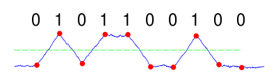
Imagine we want to send the sequence "0101100100" coded in non polar non-render-to-nothing (NRZ) through a certain channel.

Mathematically, a sequence in NRZ code tin can be described as a sequence of unit of measurement pulses or shifted rect functions, each pulse existence weighted by +1 if the bit is "1" and by -1 if the bit is "0". Formally, the scaling gene for the ${\displaystyle k^{\mathrm {th} }}$ bit is,

${\displaystyle \ a_{k}={\begin{cases}+1,&{\text{if bit }}thousand{\text{ is }}one,\\-1,&{\text{if bit }}k{\text{ is }}0.\cease{cases}}}$

We can represent our bulletin, ${\displaystyle M(t)}$ , as the sum of shifted unit pulses:

${\displaystyle \ One thousand(t)=\sum _{k=-\infty }^{\infty }a_{m}\times \Pi \left({\frac {t-kT}{T}}\right).}$

where ${\displaystyle T}$ is the fourth dimension length of i scrap.

Thus, the bespeak to exist sent by the transmitter is

If we model our noisy channel equally an AWGN channel, white Gaussian noise is added to the signal. At the receiver terminate, for a Bespeak-to-noise ratio of 3 dB, this may expect like:

A kickoff glance will not reveal the original transmitted sequence. There is a high power of noise relative to the power of the desired bespeak (i.e., there is a low indicate-to-noise ratio). If the receiver were to sample this betoken at the right moments, the resulting binary message could exist incorrect.

To increase our signal-to-noise ratio, we pass the received bespeak through a matched filter. In this instance, the filter should be matched to an NRZ pulse (equivalent to a "1" coded in NRZ lawmaking). Precisely, the impulse response of the ideal matched filter, bold white (uncorrelated) noise should be a time-reversed complex-conjugated scaled version of the signal that we are seeking. We choose

${\displaystyle \ h(t)=\Pi \left({\frac {t}{T}}\right).}$

In this instance, due to symmetry, the time-reversed circuitous cohabit of ${\displaystyle h(t)}$ is in fact ${\displaystyle h(t)}$ , allowing us to call ${\displaystyle h(t)}$ the impulse response of our matched filter convolution system.

After convolving with the right matched filter, the resulting bespeak, ${\displaystyle M_{\mathrm {filtered} }(t)}$ is,

${\displaystyle \ M_{\mathrm {filtered} }(t)=(1000*h)(t)}$

where ${\displaystyle *}$ denotes convolution.

Which can now be safely sampled past the receiver at the correct sampling instants, and compared to an appropriate threshold, resulting in a correct interpretation of the binary bulletin.

Gravitational-wave astronomy [edit]

Matched filters play a fundamental role in gravitational-wave astronomy.^[9] The first ascertainment of gravitational waves was based on large-calibration filtering of each detector's output for signals resembling the expected shape, followed past subsequent screening for ancillary and coherent triggers between both instruments. Imitation-alert rates, and with that, the statistical significance of the detection were and then assessed using resampling methods.^{[10] [11]} Inference on the astrophysical source parameters was completed using Bayesian methods based on parameterized theoretical models for the point waveform and (once again) on the Whittle likelihood.^{[12] [13]}

See likewise [edit]

• Periodogram
• Filtered backprojection (Radon transform)
• Digital filter
• Statistical signal processing
• Whittle likelihood
• Contour likelihood
• Detection theory
• Multiple comparisons problem
• Aqueduct capacity
• Noisy-aqueduct coding theorem
• Spectral density estimation
• Least hateful squares (LMS) filter
• Wiener filter
• MUltiple SIgnal Classification (MUSIC), a popular parametric superresolution method
• SAMV

Notes [edit]

1. ^ The mutual reference to SNR has in fact been criticized as somewhat misleading: "The interesting feature of this approach is that theoretical perfection is attained without aiming consciously at a maximum signal/noise ratio. As the matter of quite incidental interest, it happens that the operation [...] does maximize the peak signal/noise ratio, but this fact plays no part any in the present theory. Signal/noise ratio is not a measure of information [...]." (Woodward, 1953;^[1] Sec.five.i).

References [edit]

1. ^ ^{a b c} Woodward, P. M. (1953). Probability and data theory with applications to radar. London: Pergamon Printing.
2. ^ ^{a b} Turin, G. Fifty. (1960). "An introduction to matched filters". IRE Transactions on Data Theory. 6 (three): 311–329. doi:10.1109/TIT.1960.1057571.
3. ^ "Demodulation". OpenStax CNX . Retrieved 2017-04-18 .
4. ^ Later D.O. N who was among the start to innovate the concept: Northward, D. O. (1943). "An analysis of the factors which determine signal/racket discrimination in pulsed carrier systems". Report PPR-6C, RCA Laboratories, Princeton, NJ.
   Re-print: North, D. O. (1963). "An analysis of the factors which determine point/dissonance bigotry in pulsed-carrier systems". Proceedings of the IEEE. 51 (7): 1016–1027. doi:10.1109/PROC.1963.2383.
   See also: Jaynes, Due east. T. (2003). "14.half dozen.1 The classical matched filter". Probability theory: The logic of science. Cambridge: Cambridge Academy Press.
5. ^ Choudhuri, Due north.; Ghosal, Southward.; Roy, A. (2004). "Contiguity of the Whittle measure out for a Gaussian time series". Biometrika. 91 (4): 211–218. doi:10.1093/biomet/91.1.211.
6. ^ Mood, A. G.; Graybill, F. A.; Boes, D. C. (1974). "9. Tests of hypotheses". Introduction to the theory of statistics (3rd ed.). New York: McGraw-Hill.
7. ^ ^{a b c} Röver, C. (2011). "Student-t based filter for robust bespeak detection". Physical Review D. 84 (12): 122004. arXiv:1109.0442. Bibcode:2011PhRvD..84l2004R. doi:ten.1103/PhysRevD.84.122004.
8. ^ Neyman, J.; Pearson, E. Due south. (1933). "On the problem of the well-nigh efficient tests of statistical hypotheses". Philosophical Transactions of the Purple Gild of London A. 231 (694–706): 289–337. Bibcode:1933RSPTA.231..289N. doi:10.1098/rsta.1933.0009.
9. ^ Schutz, B. F. (1999). "Gravitational wave astronomy". Classical and Quantum Gravity. 16 (12A): A131–A156. arXiv:gr-qc/9911034. Bibcode:1999CQGra..16A.131S. doi:10.1088/0264-9381/16/12A/307.
10. ^ Usman, Samantha A. (2016). "The PyCBC search for gravitational waves from compact binary coalescence". Class. Breakthrough Grav. 33 (21): 215004. arXiv:1508.02357. Bibcode:2016CQGra..33u5004U. doi:10.1088/0264-9381/33/21/215004.
11. ^ Abbott, B. P.; et al. (The LIGO Scientific Collaboration, the Virgo Collaboration) (2016). "GW150914: First results from the search for binary black pigsty coalescence with Avant-garde LIGO". Physical Review D. 93 (12): 122003. arXiv:1602.03839. Bibcode:2016PhRvD..93l2003A. doi:x.1103/PhysRevD.93.122003. PMC7430253. PMID 32818163.
12. ^ Abbott, B. P.; et al. (The LIGO Scientific Collaboration, the Virgo Collaboration) (2016). "Properties of the binary black hole merger GW150914". Physical Review Letters. 116 (24): 241102. arXiv:1602.03840. Bibcode:2016PhRvL.116x1102A. doi:10.1103/PhysRevLett.116.241102. PMID 27367378.
13. ^ Meyer, R.; Christensen, Due north. (2016). "Gravitational waves: A statistical autopsy of a blackness pigsty merger". Significance. 13 (2): 20–25. doi:x.1111/j.1740-9713.2016.00896.x.

Further reading [edit]

• Turin, M. Fifty. (1960). "An introduction to matched filters". IRE Transactions on Information Theory. half dozen (3): 311–329. doi:ten.1109/TIT.1960.1057571.
• Wainstein, Fifty. A.; Zubakov, V. D. (1962). Extraction of signals from noise. Englewood Cliffs, NJ: Prentice-Hall.
• Melvin, W. Fifty. (2004). "A STAP overview". IEEE Aerospace and Electronic Systems Magazine. 19 (1): 19–35. doi:10.1109/MAES.2004.1263229.
• Röver, C. (2011). "Student-t based filter for robust signal detection". Physical Review D. 84 (12): 122004. arXiv:1109.0442. Bibcode:2011PhRvD..84l2004R. doi:ten.1103/PhysRevD.84.122004.
• Fish, A.; Gurevich, Southward.; Hadani, R.; Sayeed, A.; Schwartz, O. (December 2011). "Computing the matched filter in linear fourth dimension". arXiv:1112.4883 [cs.IT].

What Is A Matched Filter,

Source: https://en.wikipedia.org/wiki/Matched_filter

Posted by: powellwereft.blogspot.com

Share this post